Photometry
In this tutorial, we will explore the capabilities of Siril to perform photometric processing to display a light curve of a variable star. And in this example, the variability of the star comes from a transit of an exoplanet.
EPIC-211089792 b, an exoplanet in Taurus, discovered in 2016 #
Plate solving #
Courtesy of Gerard Arlic, one of the co-discoverers of EPIC-211089792 b under the direction of the astrophysicist A. Santerne, I have in my hands a set of 111 images containing a transit of the planet, a hot Jupiter, in front of the star WASP-152. These images are excellent as an example and represent the best of the pro-am collaboration. The scientific paper of its discovery can be found here
.
The WASP-152 sequence loaded in Siril With trial and error, we can find parameters for which the plate solving suceeds. It could be useful to untick the 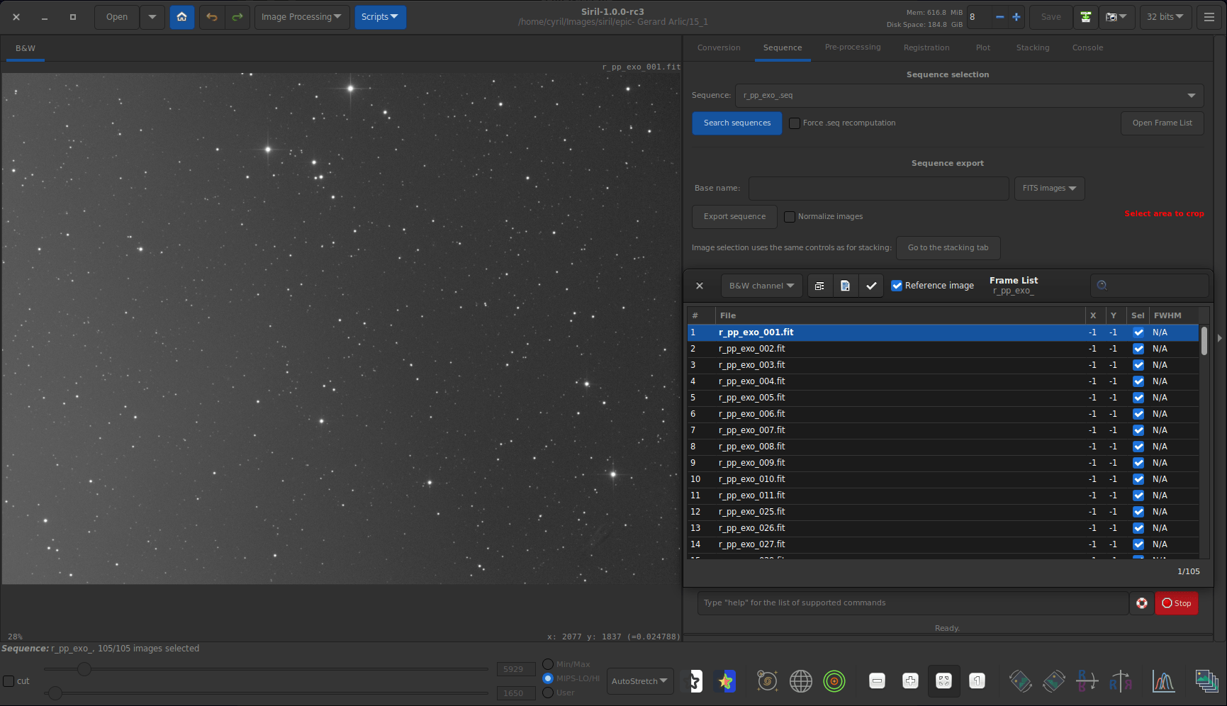
Image Plate Solver tool of Siril is in this case a very good friend. For this sequence of images, I don’t know the focal length nor the pixel size, which are input data for the tool. We will have to find them by guessing, trying various values until it works, for example by setting an arbitrary pixel size and modifying the focal length at each try. Quickly we got the result shown below. It was done on the first image of the sequence.
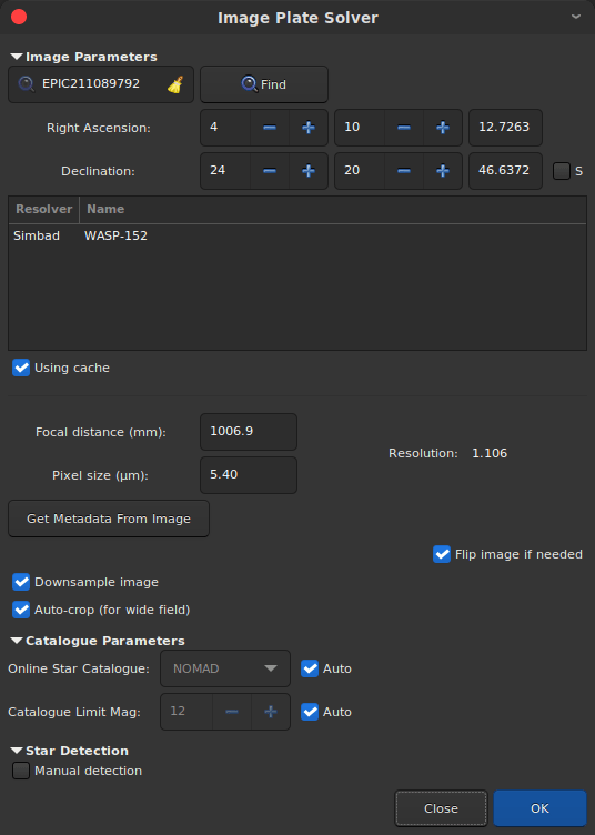
Flip Image if Needed option when images are mirrored in order to preserve orientation.
20:17:50: Findstar: processing...
20:17:50: Catalog PPMXL size: 843 objects
20:17:50: 82 pair matches.
20:17:50: Inliers:         0.585
20:17:50: Resolution:      1.106 arcsec/px
20:17:50: Rotation:     +179.92 deg
20:17:50: Focal:        1006.88 mm
20:17:50: Pixel size:      5.40 µm
20:17:50: Field of view:    01d 01m 56.91s x 46' 45.38"
20:17:50: Image center: alpha:  04h10m13s, delta: +24°20'47"
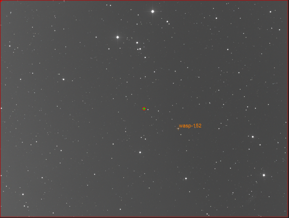
Now that the plate solving succeeded, we have access to a lot of interesting features. Here we will use the object search, available in the context menu of the image (right click on it), the We input again the name of the variable star. The variable star is now annotated.Search Object... entry (also available as control+shift+/). A small dialog box opens, in which we’ll type WASP-152 (or EPIC-211089792) and Enter.

WASP-152 becomes annotated, and this will help us greatly for the analysis.
Photometry of the sequence #
Now that we know where to find the star, we will start analysing it. First, the images have to be aligned, in case they show some movement between each other, to facilitate the analysis of the same star in all images.
This will be very easy in our example since we have a lot of visible stars in the images, we can use the Two-Pass Global Star Alignment (deep-sky) algorithm.
This method has 2 main assets:
- First, one can save a lot of space on the disk since no new image is created. All the registration data are stored in the existing
.seqfile. - Second, as no new image is generated, no unwanted interpolation between pixel values occur, and we keep the images as pristine as possible.
Aligning images is a key step for sequence photometry analysis.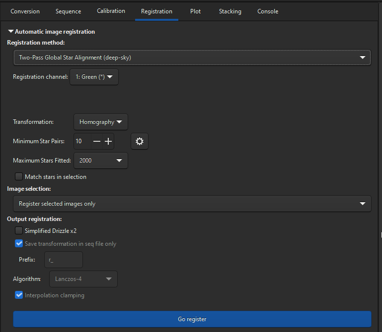
20:22:01: Sequence processing succeeded.
20:22:01: Execution time: 36.52 s.
20:22:01: Registration finished.
20:22:01: 111 images processed.
20:22:01: Total: 0 failed, 111 registered.
Before getting to the heart of the matter, with photometry, it is advisable to go to the The dot cloud represents the wFWHM as a function of the roundness of the stars. It is easy to identify the points (images) that cause problems.Graphics tab in order to analyze the images and to deselect those likely to cause problems in the analysis. The latest versions of Siril have a formidable tool for this, with the possibility of displaying several selection criteria depending on the others. In particular, after a global alignment it is possible to display the FWHM with regards to the roundness of the stars. In the following illustration, I even chose to use the wFWHM which is an improved FWHM.

Once all images aligned and sorted, we can actually analyse the photometry of the sequence.
First, you have to set the Photometry mode by toggling the dedicated button:
To set the Photometry mode.
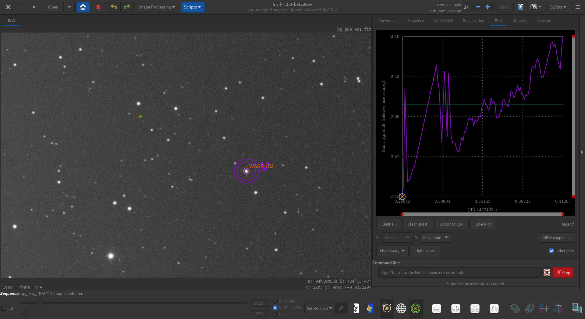
Let’s start with the variable star. By right clicking on it, the apertures used for photometry calculation are drawn and a PSF computation is done on the whole sequence.
Photometry is done on the variable star for all images of the sequence. Uncalibrated magnitude plot for the variable star.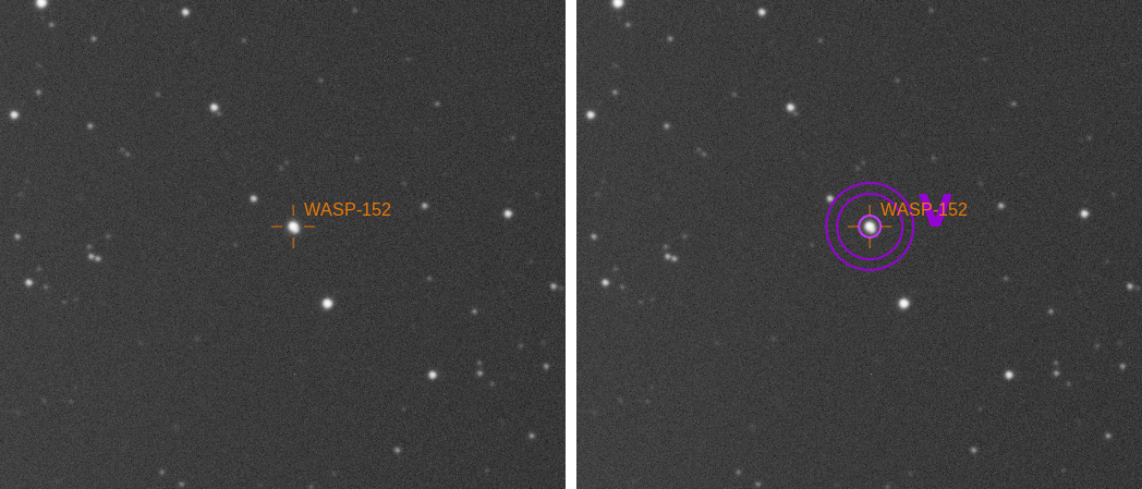
Cancel last button.
Ideally, stars whose magnitude is stable across the sequence must be selected. If nearby stars are unknown, another feature is very useful:
- Unset the Photometry mode by toggling the button.
- Select a star.
- Context menu (right click) ->
PSF(not for the sequence this time) - Click on
More details...in the new window - This opens a Web browser page with data on the selected star.
Here, for learning purposes, I didn’t push the analysis as far as finding stable stars in the image, and took 4 random stars. The variable star is variable enough for a probable good result any way. When choosing the reference stars, it is also a good idea to select stars whose brightness is alike the variable’s, that are not too far from it, especially if flat field correction is not done (it should be mandatory for this kind of analysis), and not on the borders of images in case there is some shift between them. After choosing the reference stars, run the sequence photometric analysis on each star.
It’s interresting to set the X axis as Julian date rather than frame number.
Four reference stars have been chosen in the image. Light curve of 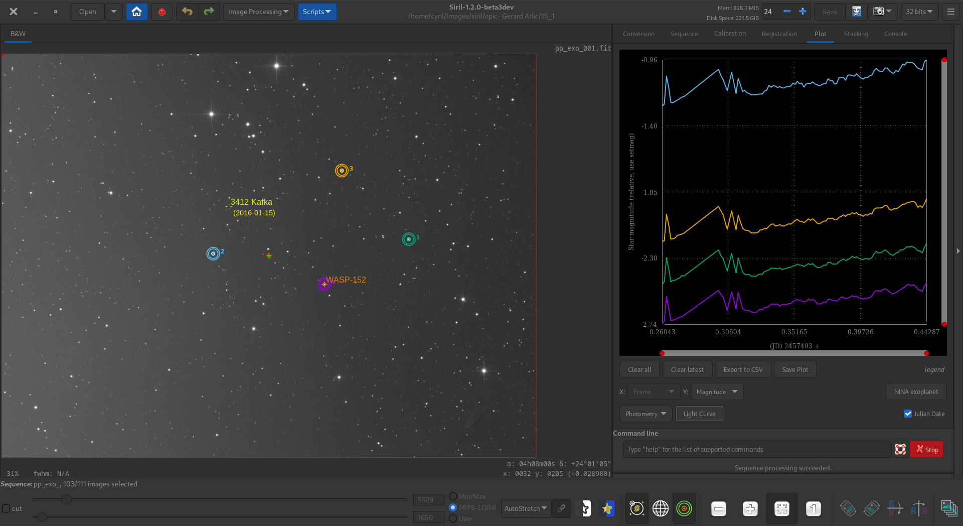
Light curve button becomes active, and clicking on it allows, as its name suggests, the light curve of the variable star to be plotted. A data file is saved, useful if the analysis is to be shared or for further analysis. If gnuplot
is installed, this will automatically display the light curve plot.
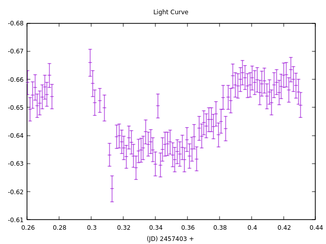
WASP-152. We clearly see a dip indicating the transit of the exoplanet.
We have just seen how, in a simple way, Siril allows to make a photometric study of an exoplanet transit. Obviously, this method is applicable to many other objects such as variable stars, occultation of stars by an asteroid, etc … We encourage you to try the adventure and to share your results.